
-
Tight Smoothing of Singular Functions
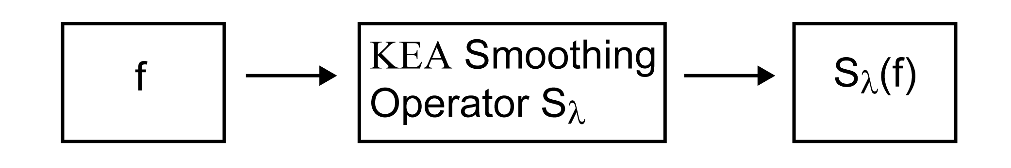
- The present operator performs a tight smoothing on the input function. Let ƒ be a scalar function of any number of variables, which can be not continuous or nor smooth, that is,
ƒ can be continuous but not continuously differentiable, the smoothing operator
when applied to ƒ will return a smooth function which is equal to the input function
ƒ apart from a neighborhood of the singularities of ƒ. The width of the neighbourhood is controlled by a parameter l. The larger is
l, the smaller is the neighborhood. For l → +∞, Slƒ
→ ƒ, whereas for l → 0, Slƒ → co(ƒ), convex envelope of ƒ.
- EXAMPLES:
- For illustration purpose, the KEA Smoothing Method is next displayed for scalar functions of two variables.
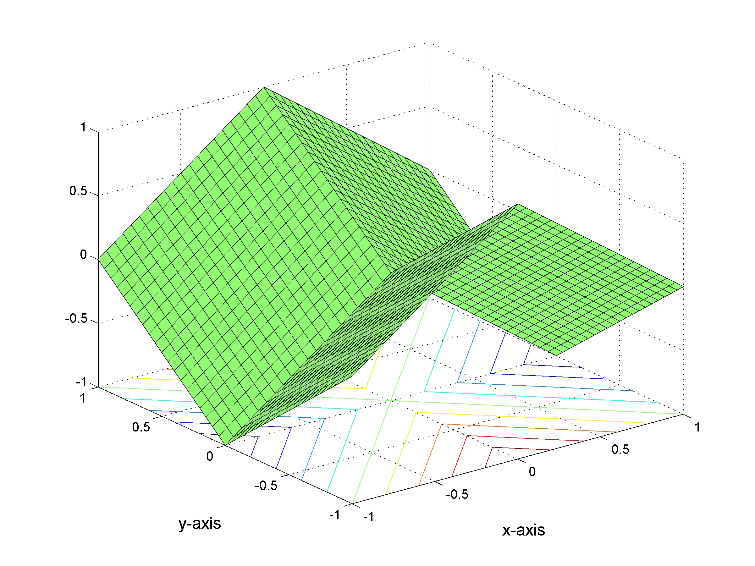
- i) ƒ(x,y)=|x|-|y|
- ii) ƒ(x,y)=0.05(sign(x)+sign(y))
- i) Tight Smoothing of ƒ(x,y)=|x|-|y|
-
 (a)
(a)
 (b)
(b)
- (a) Graph of ƒ for x ∈ [-1,1] and y ∈ [-1,1], together with the isolevel curves of ƒ, that is, curves of equation ƒ(x,y)=k with k∈R. Observe that ƒ is not smooth along the lines of equation x=0 and y=0.
-
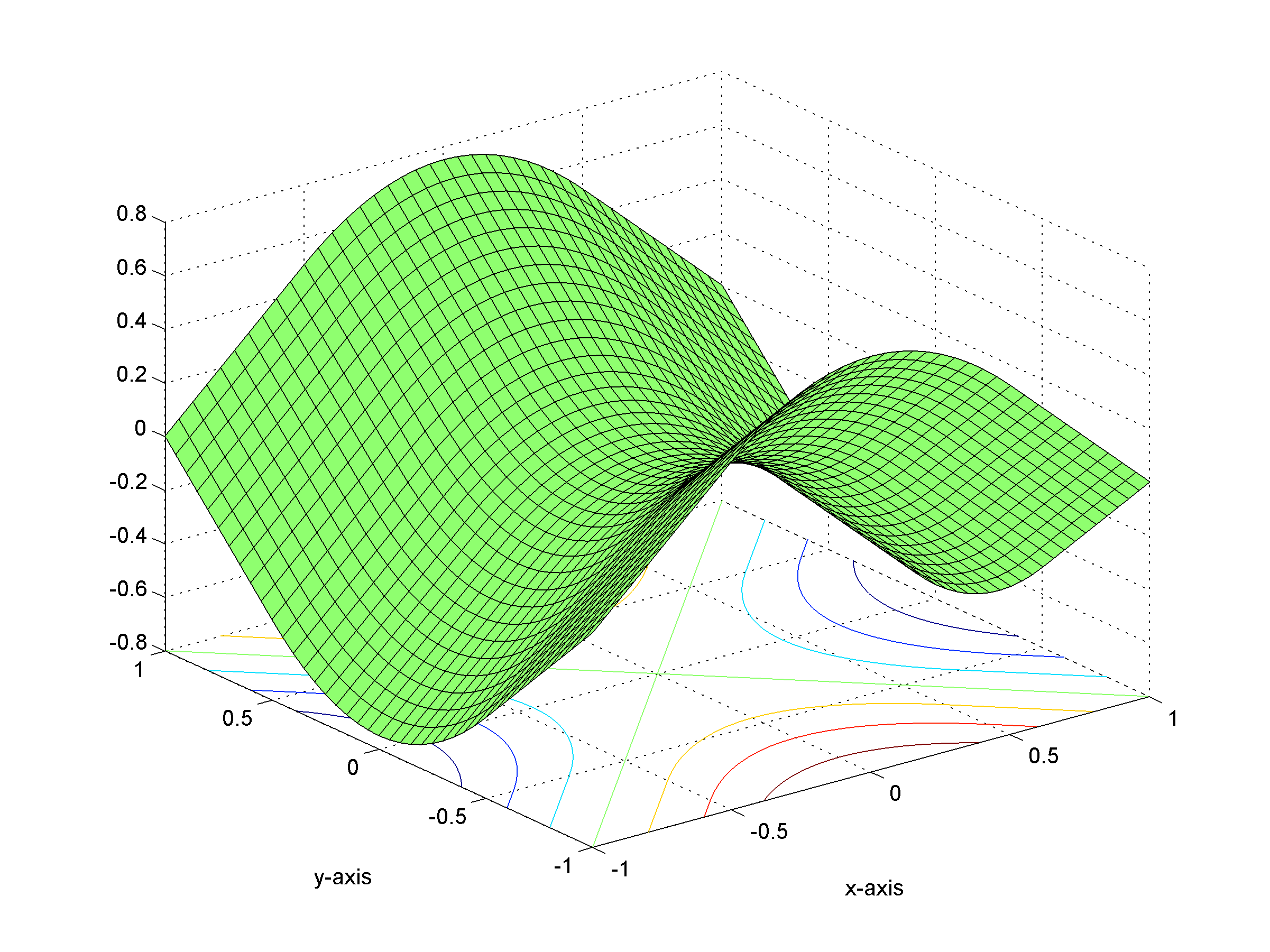
(b) Graph of the tight approximation Slƒ of ƒ for l=1. Observe that Slƒ is now smooth along the lines of equation x=0 and y=0.

-
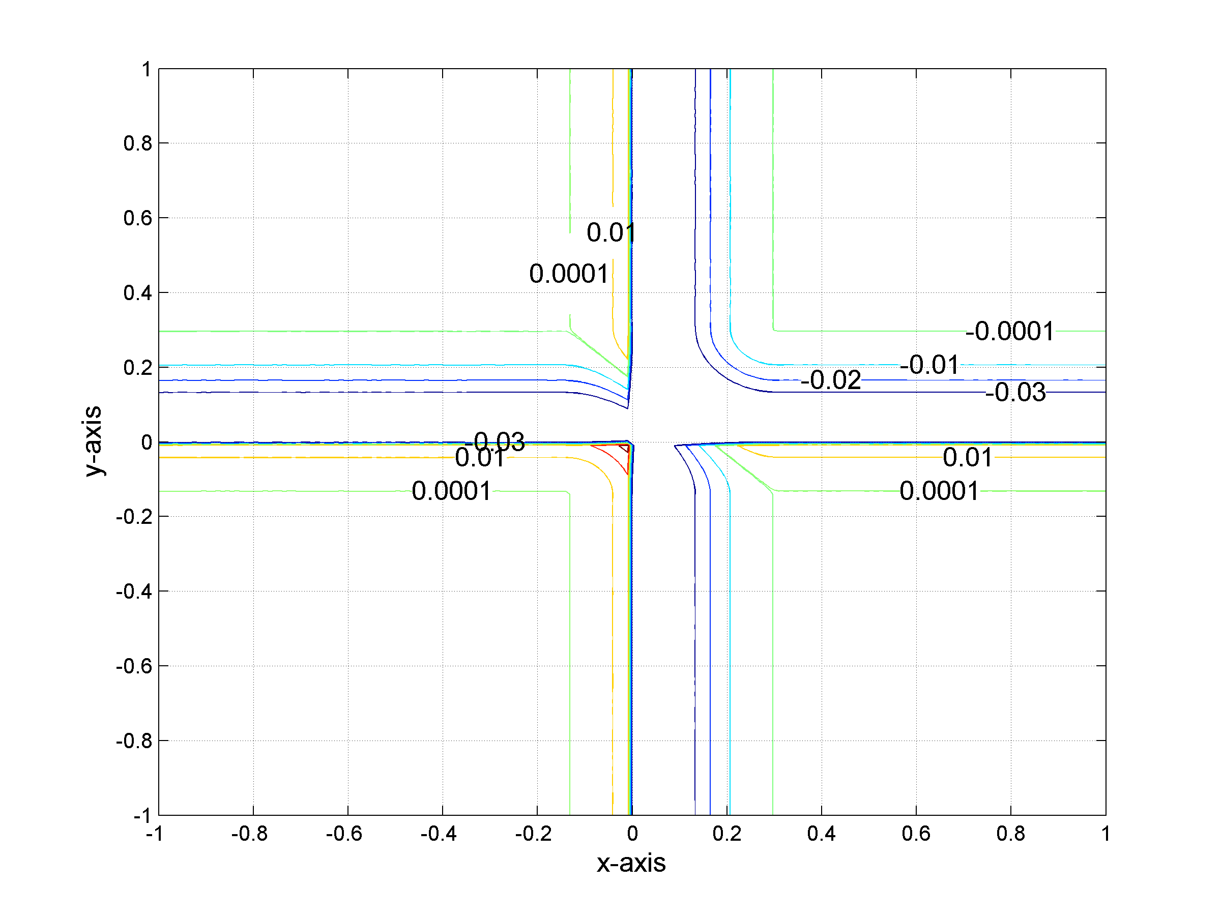
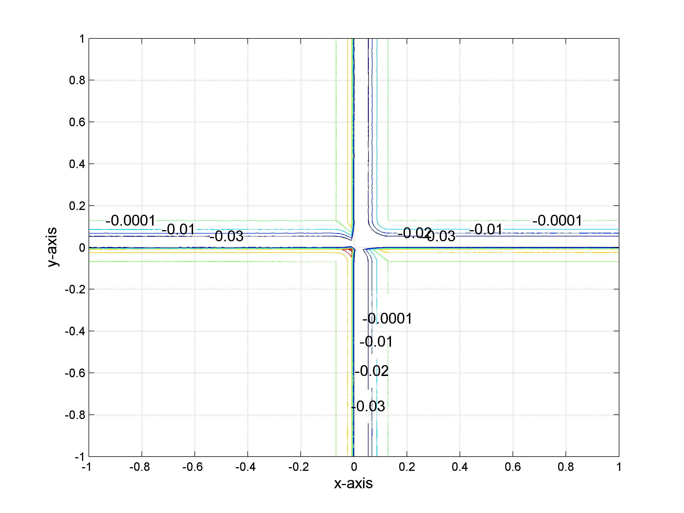
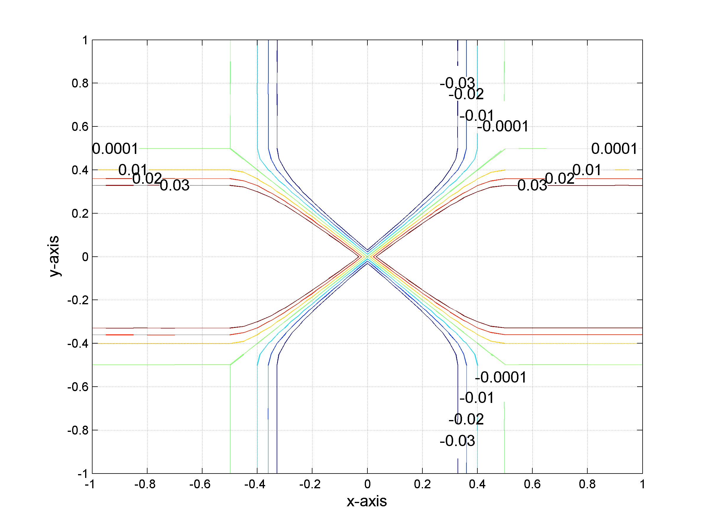 Isolevels of the difference between ƒ and the tight approximation Slƒ of ƒ for l=1. The difference is zero everywhere apart from a neighborhood of the lines of equation x=0 and y=0. The width of the neighbourhood is controlled by the parameter l.
-
 (a)
(a)
 (b)
(b)
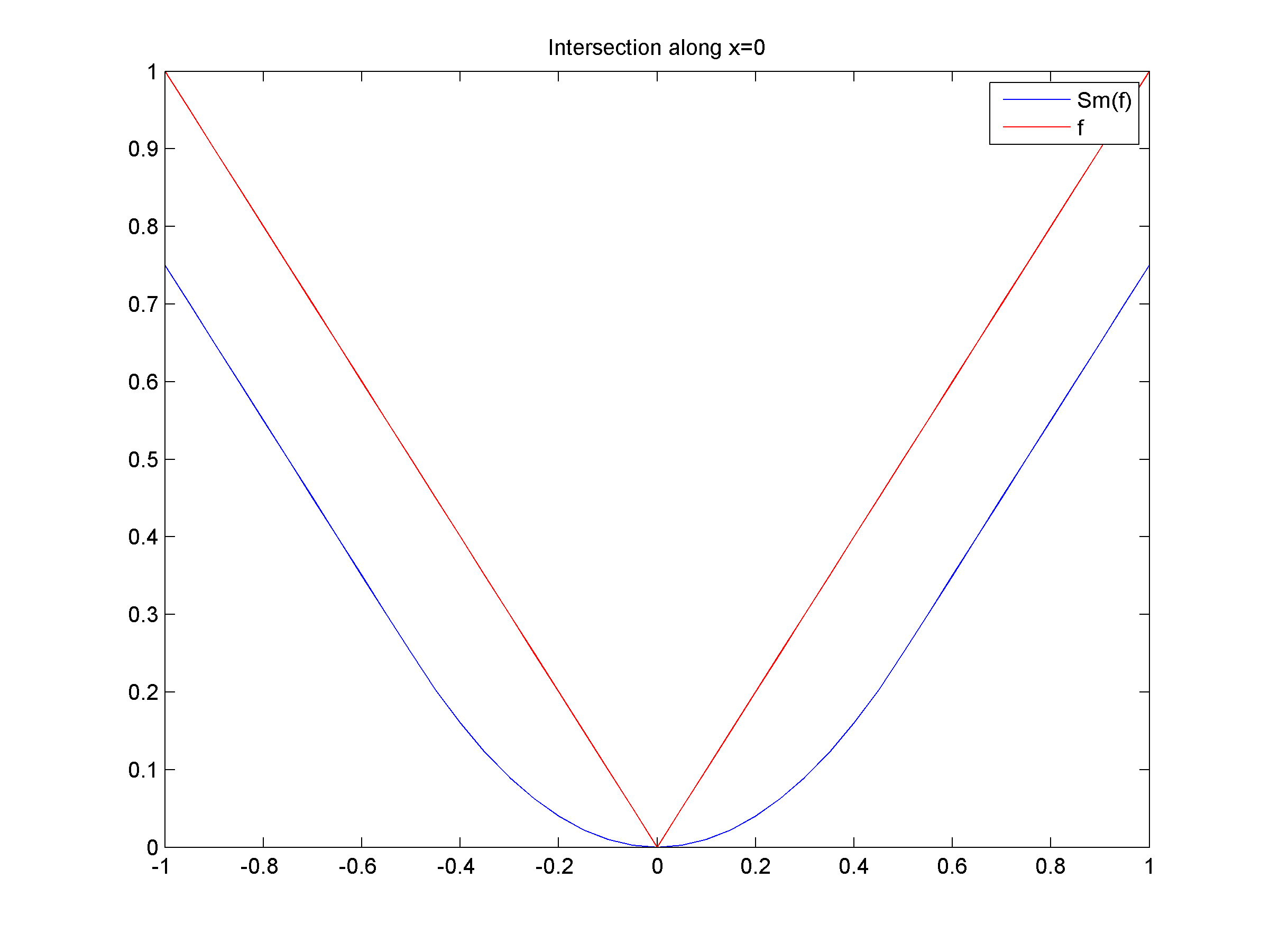
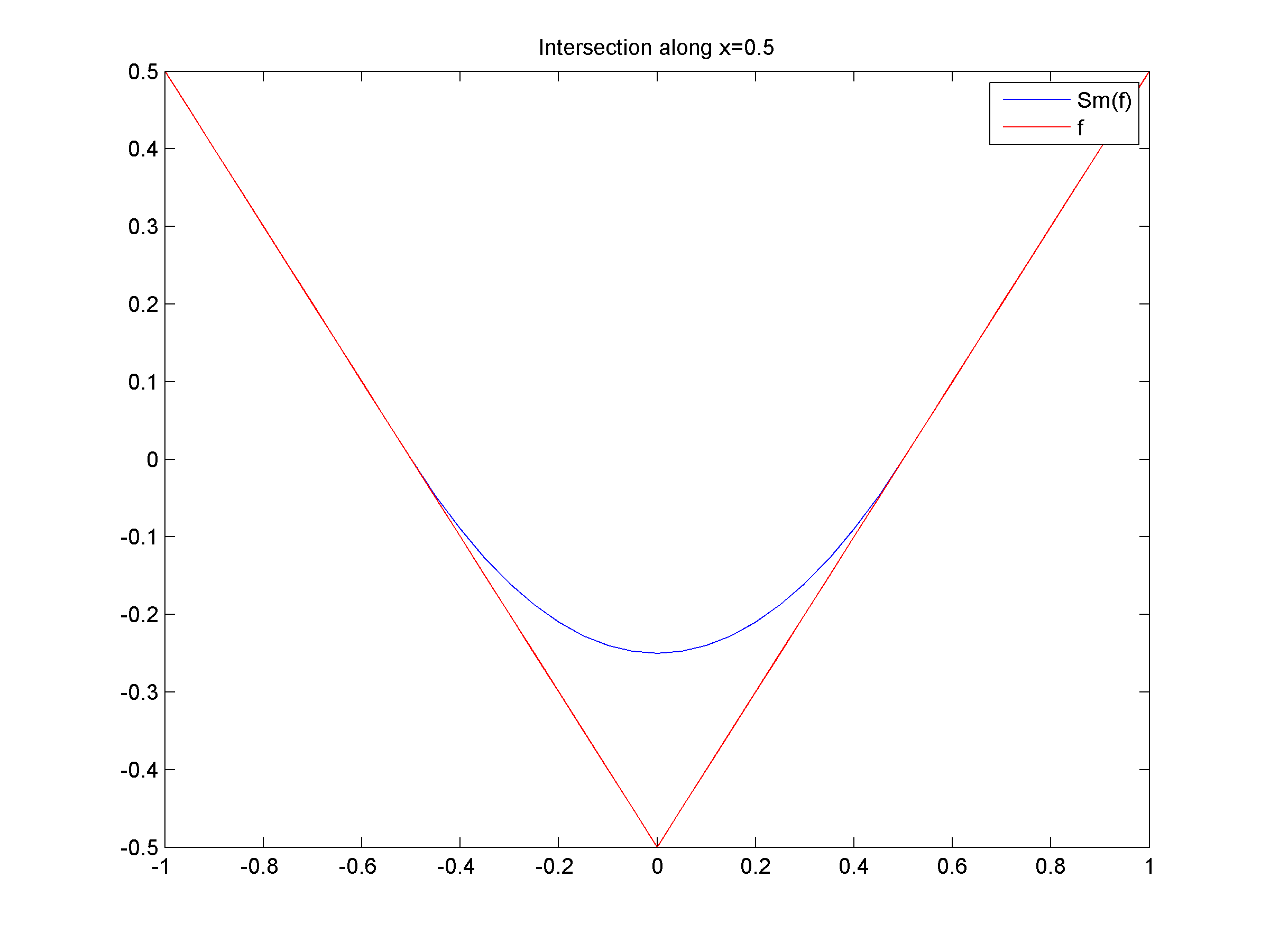
- Cross sections of ƒ and Slƒ at (a) x=0 and (b) x=0.5.
-
 (a)
(a)
 (b)
(b)
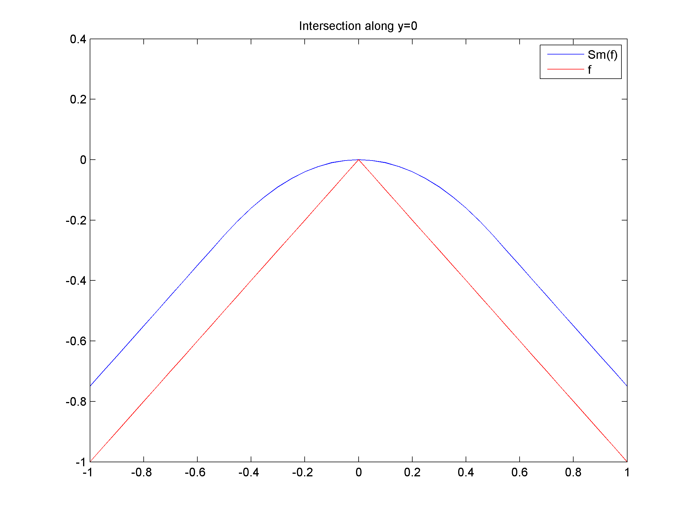
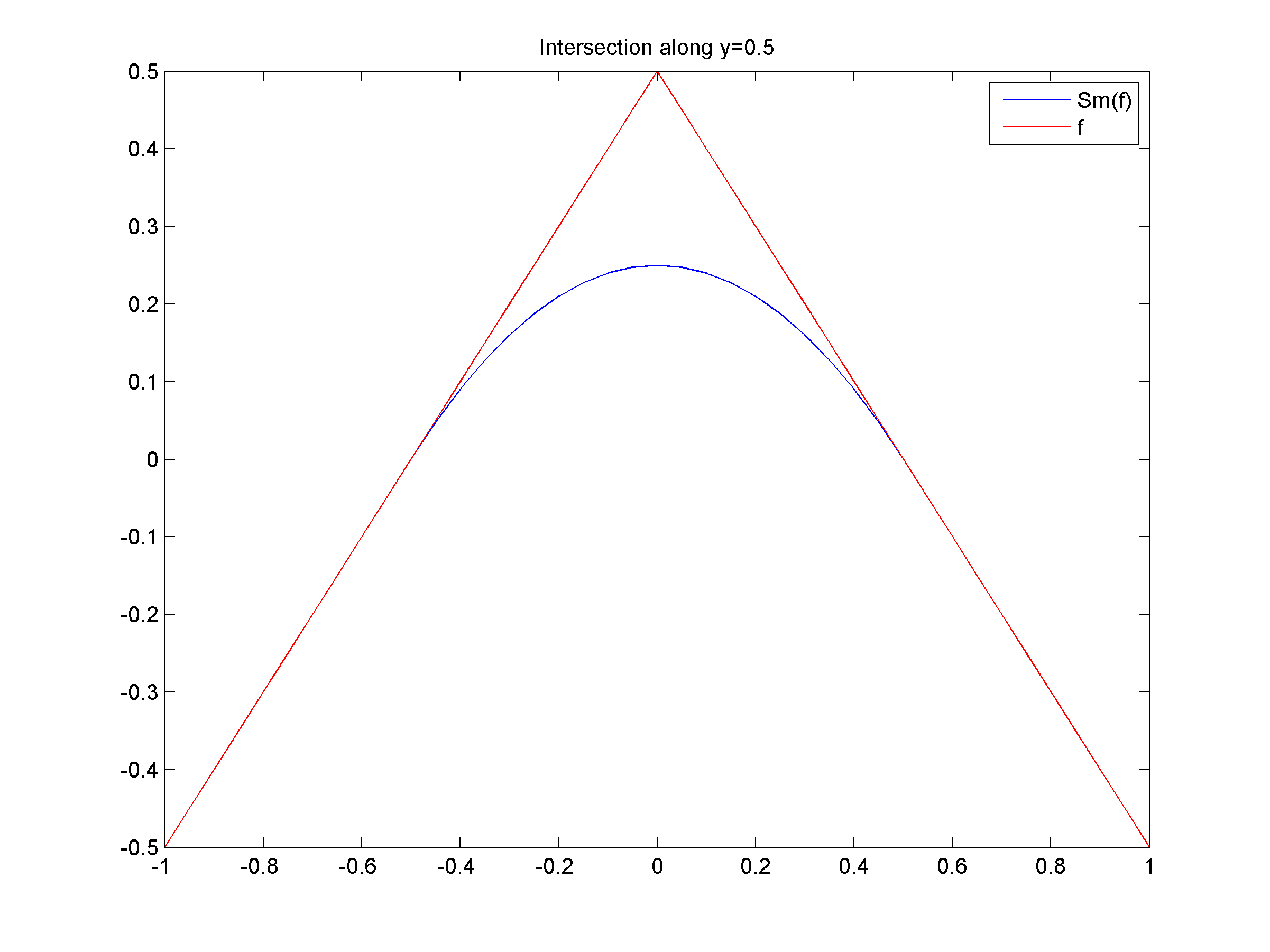
- Cross sections of ƒ and Slƒ at (a) y=0 and (b) y=0.5.
-
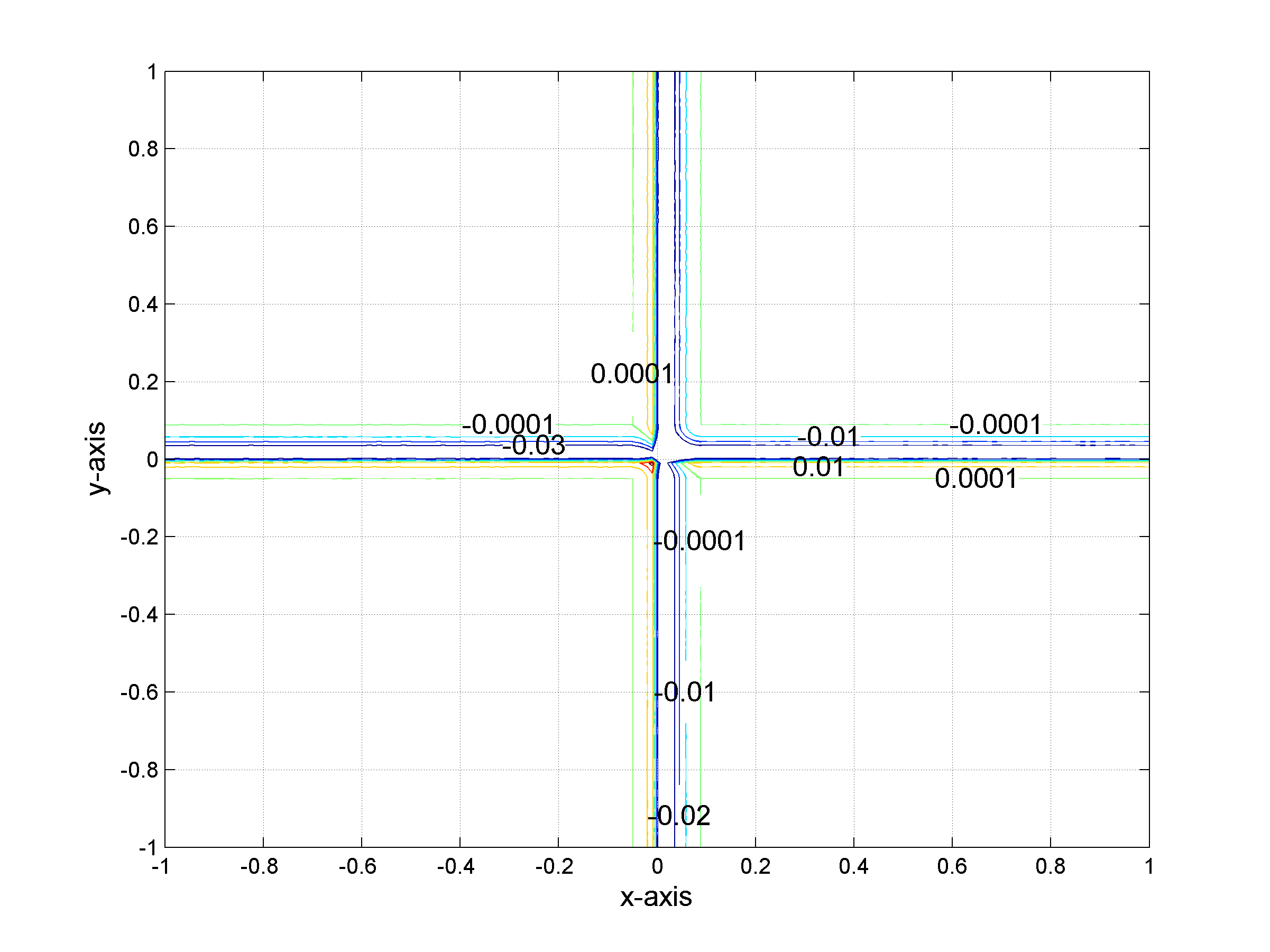
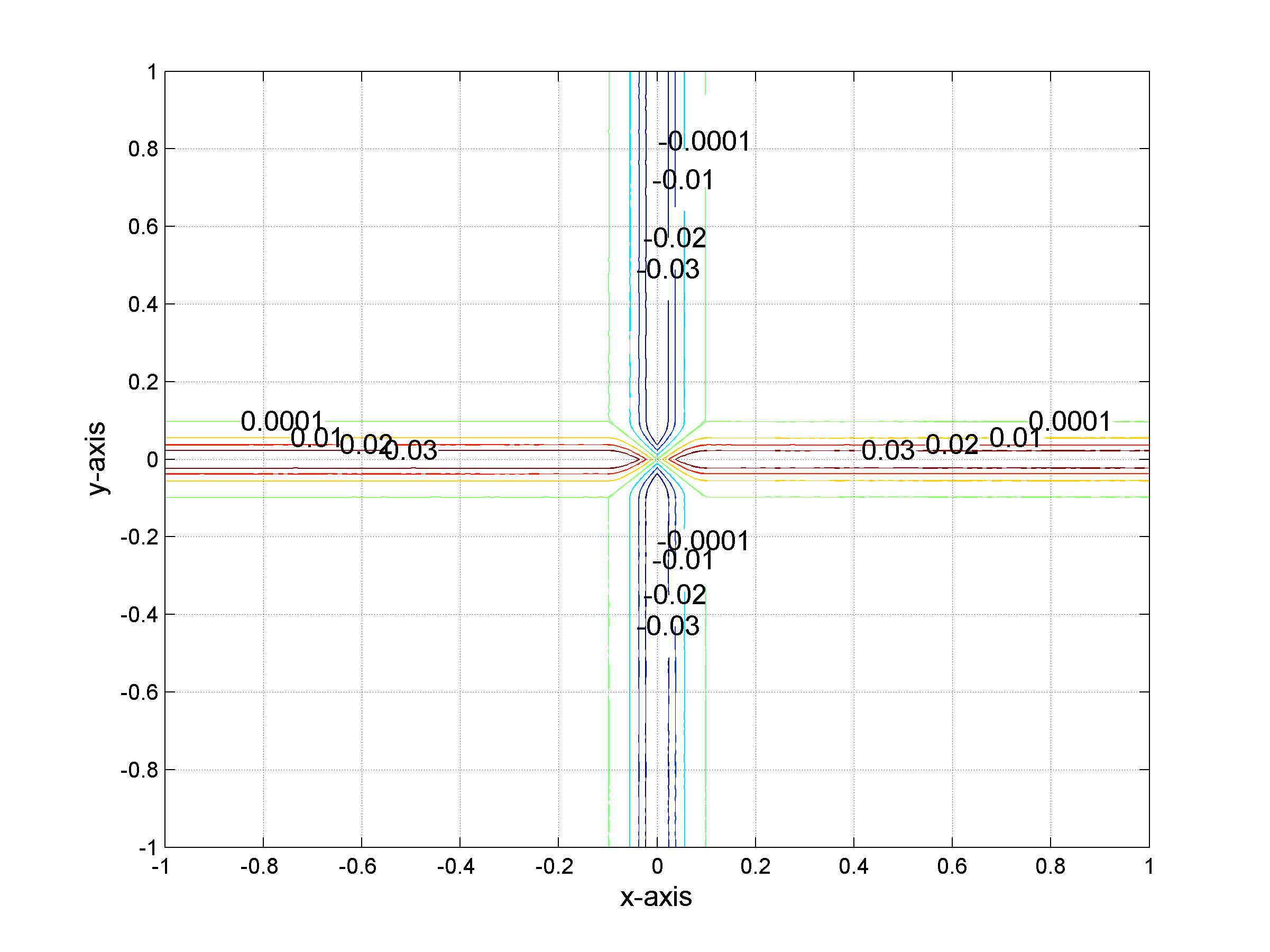 Isolevels of the difference between ƒ and the tight approximation Slƒ of ƒ for l=5.
-
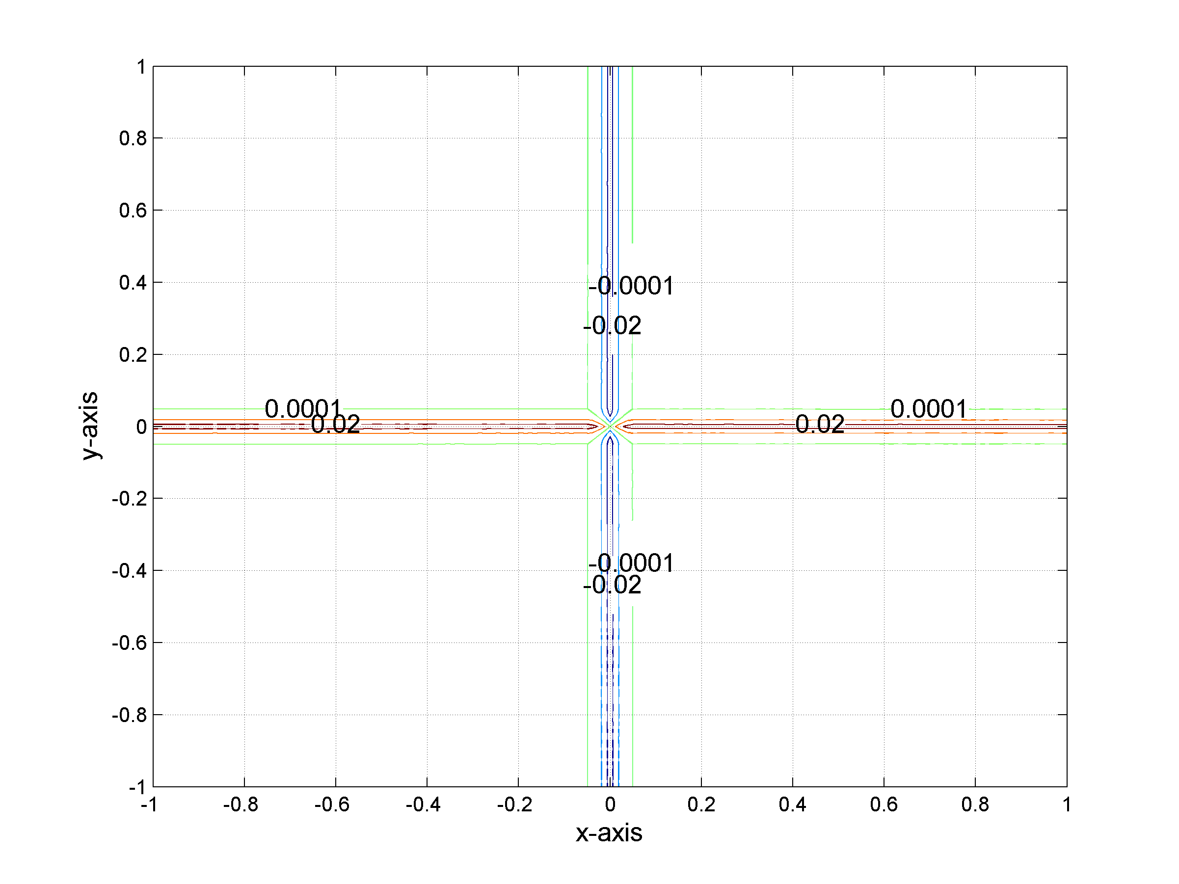 Isolevels of the difference between ƒ and the tight approximation Slƒ of ƒ for l=10.
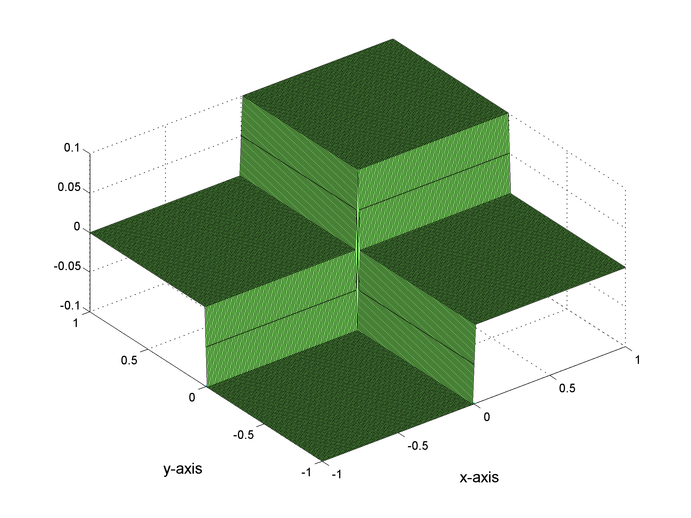
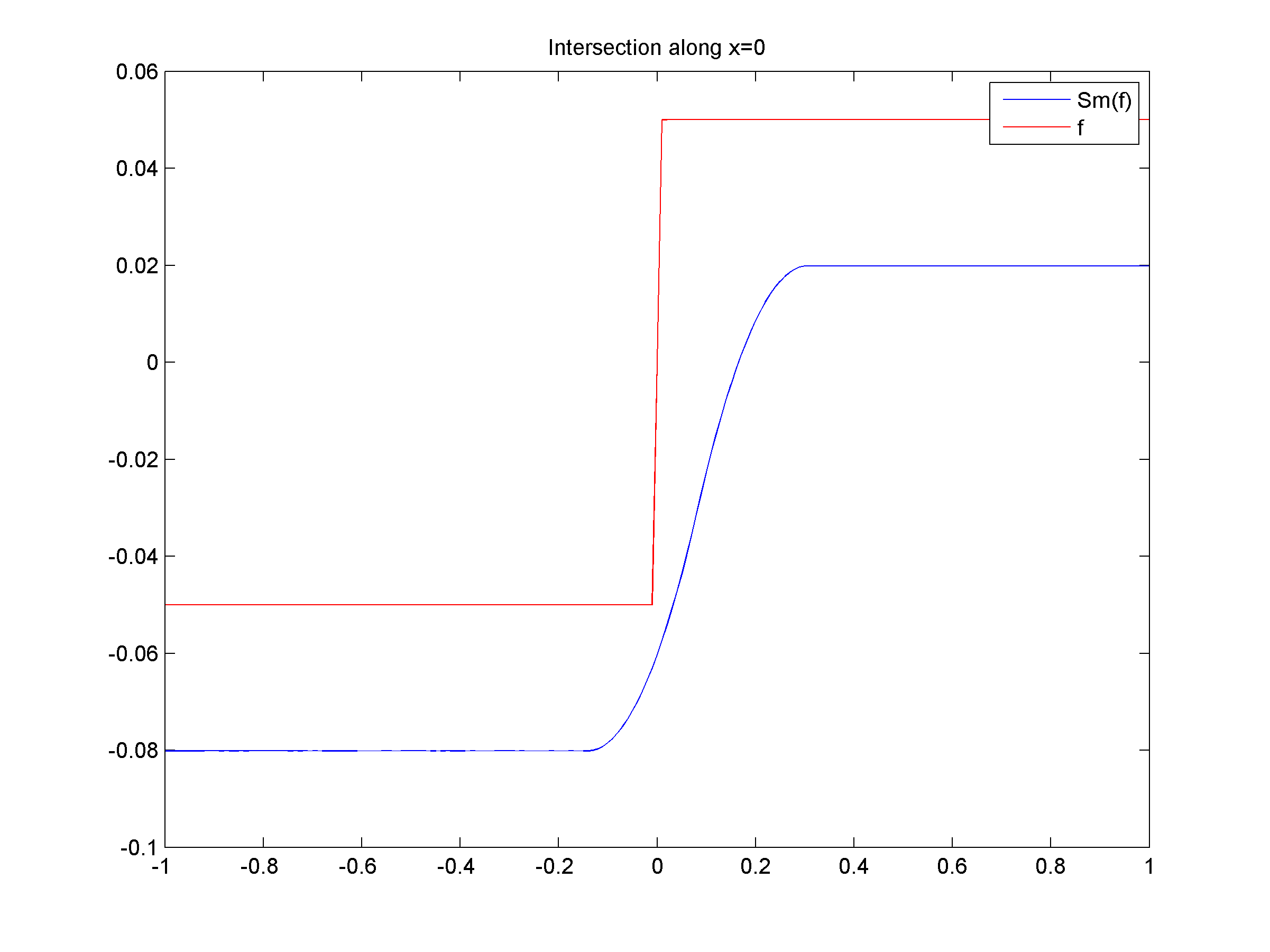
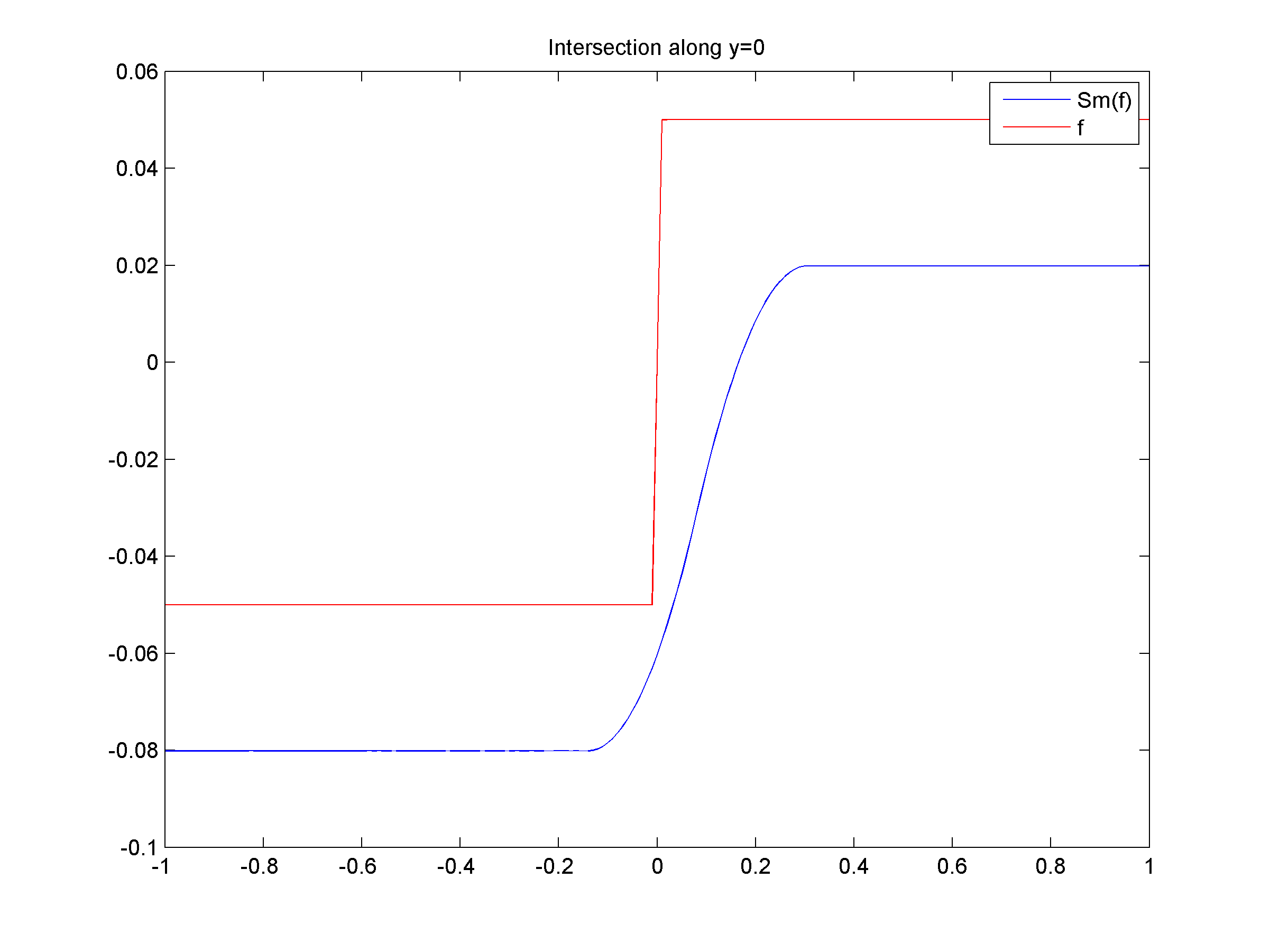
- ii) Tight Smoothing of ƒ(x,y)=0.05(sign(x)+sign(y))
-
 (a)
(a)
 (b)
(b)
- (a) Graph of ƒ with x ∈ [-1,1] and y ∈ [-1,1], together with the isolevel curves of ƒ, that is, curves of equation ƒ(x,y)=k with k∈R. Observe that ƒ is not smooth along the lines of equation x=0 and y=0.
-
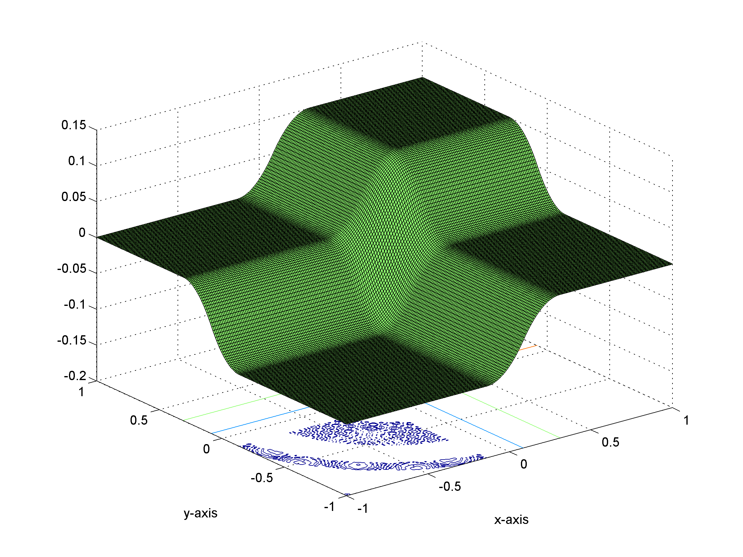
(b) Graph of the tight approximation Slƒ of ƒ for l=1. Observe that Slƒ is now smooth along the lines of equation x=0 and y=0.
-
 Isolevels of the difference between ƒ and the tight approximation Slƒ of ƒ for l=1. The difference is zero everywhere apart from a neighborhood of the lines of equation x=0 and y=0. The width of the neighbourhood is controlled by the parameter l.
-
 (a)
(a)
 (b)
(b)
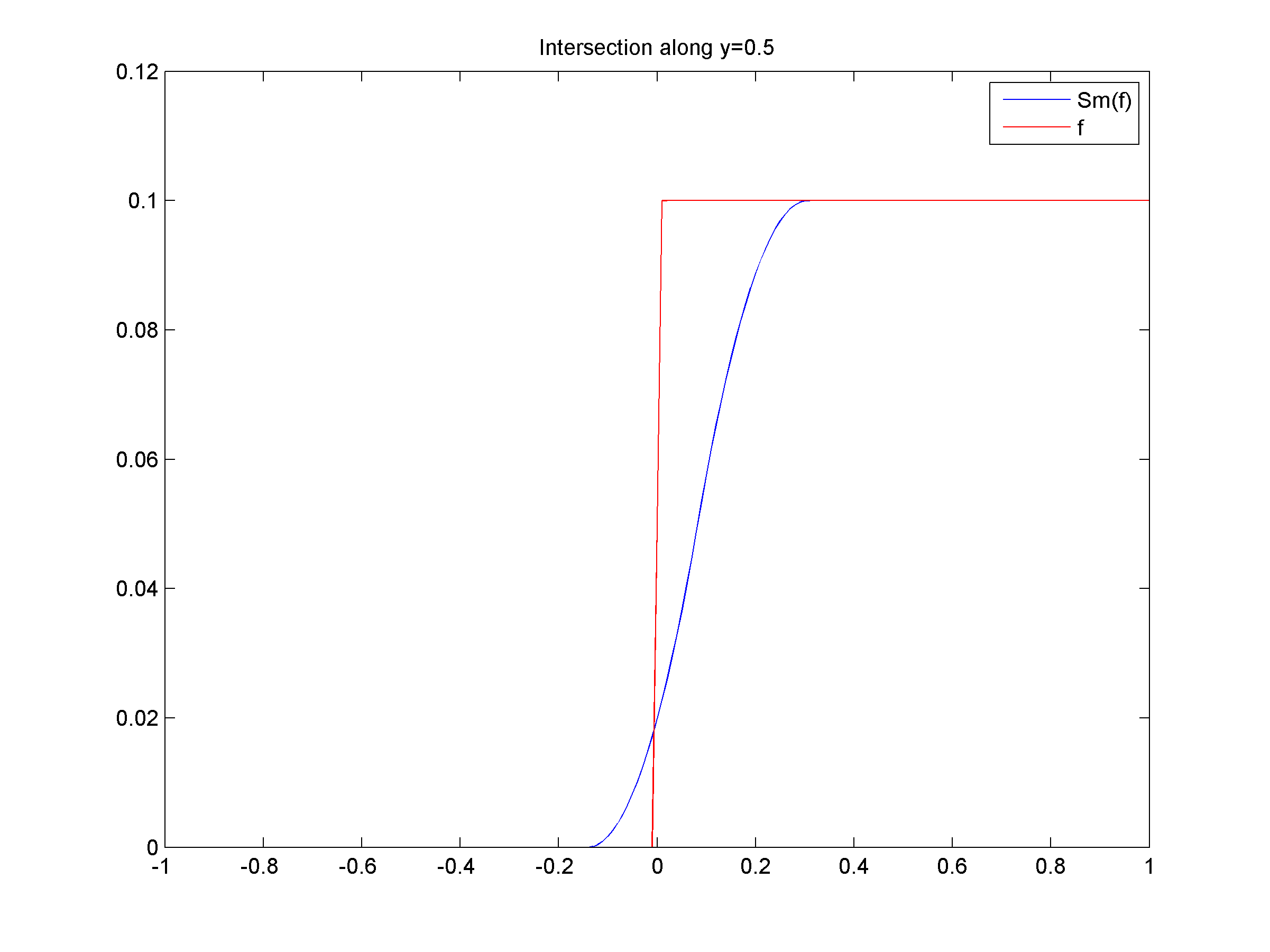
- Cross sections of ƒ and Slƒ at (a) x=0 and (b) x=0.5.
-
 (a)
(a)
 (b)
(b)
- Cross sections of ƒ and Slƒ at (a) y=0 and (b) y=0.5.
-
 Isolevels of the difference between ƒ and the tight approximation Slƒ of ƒ for l=5.
-
 Isolevels of the difference between ƒ and the tight approximation Slƒ of ƒ for l=10.