KEA Image and Data Processing, Analysis & Computational Geometry

Edge Detection

EXAMPLES:

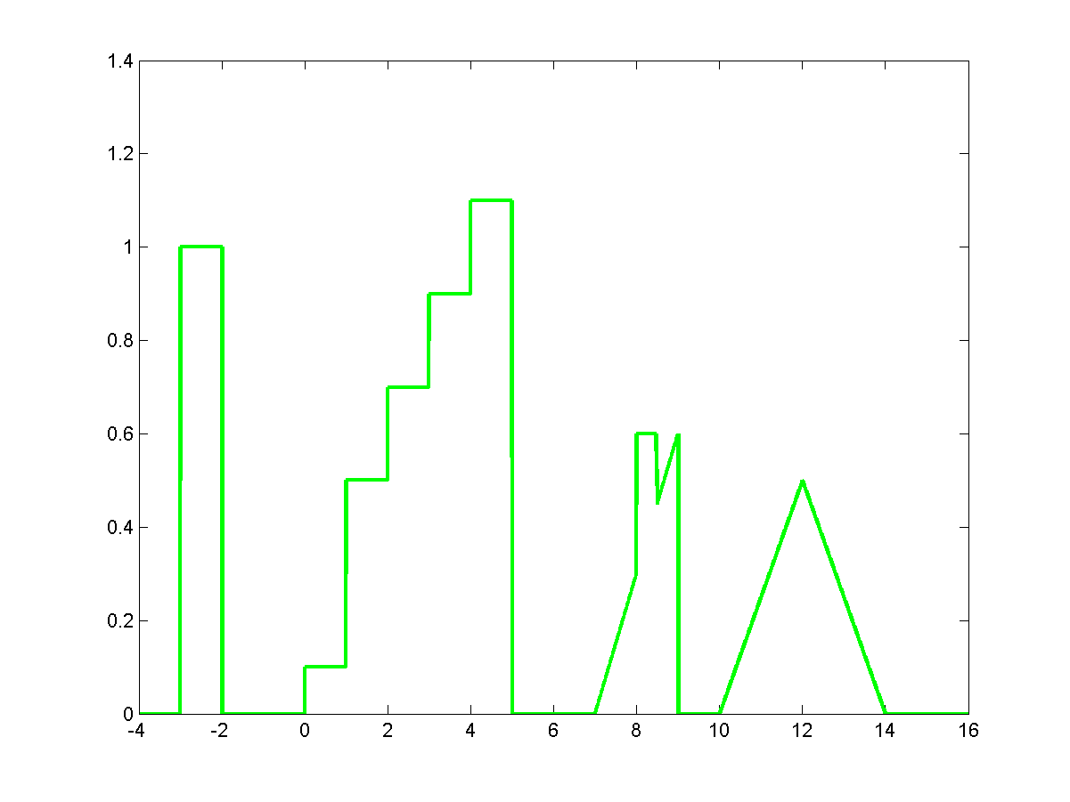
i) 1d signal with different edge types
(a)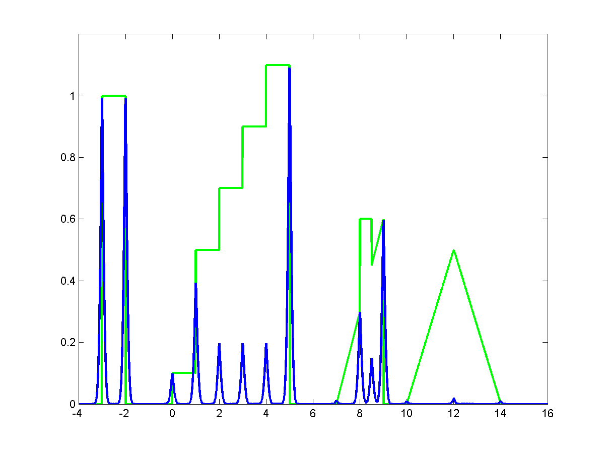

(b)
(c)
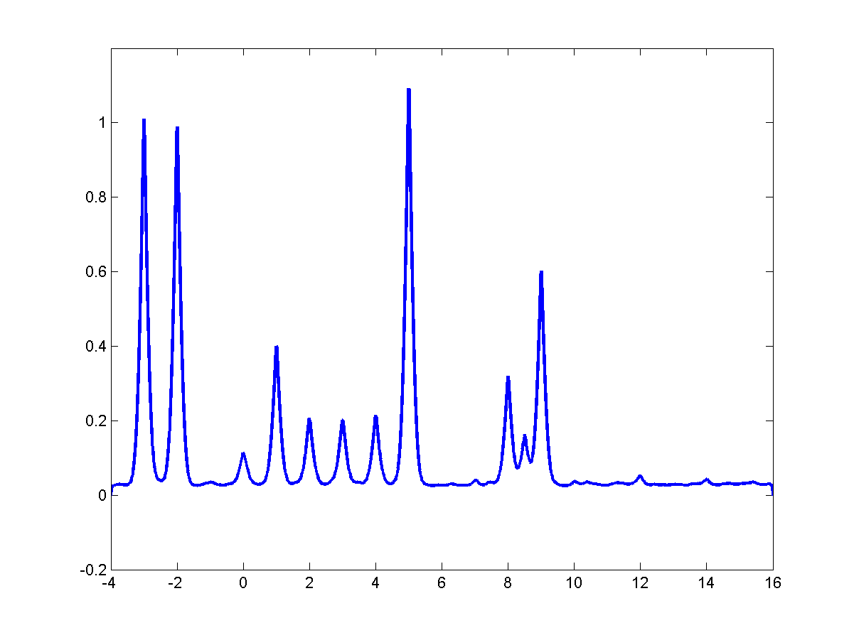
- (a) Input signal with various edge types.
- (b) Edge map displayed superimposed to the input signal.
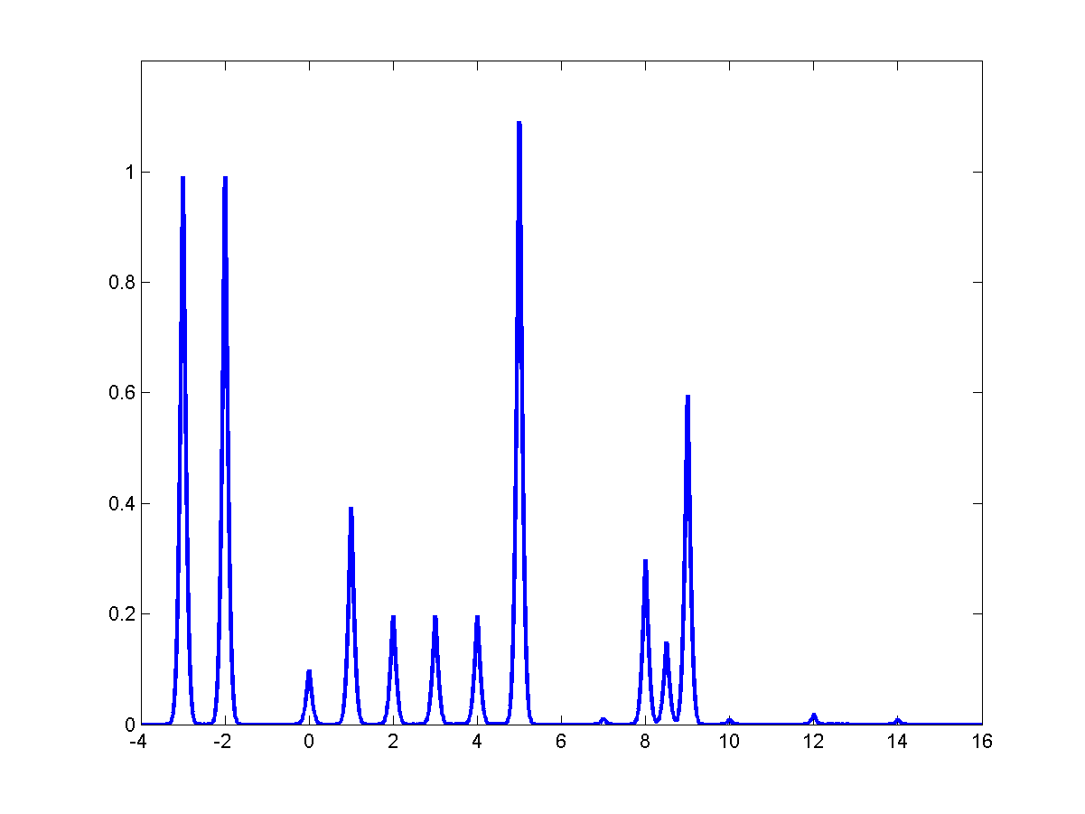
- (c) Edge map corresponding to l=0.1 and it =10⁴.

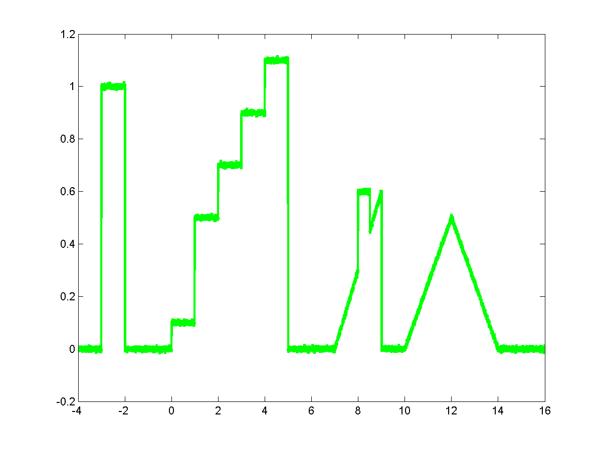
ii) 1d signal with different edge types and with Gaussian noise
(a)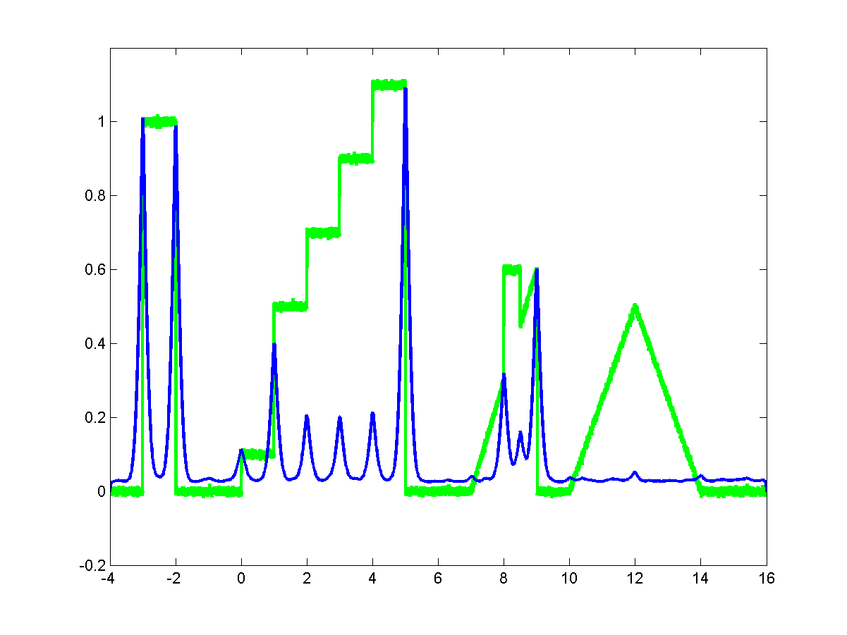

(b)
(c)
- (a) Input signal with various edge types and with Gaussian noise.
- (b) Edge map displayed superimposed to the input signal.
- (c) Edge map corresponding to l=10^-8 and it =2.5∙10⁴.

iii) SUSAN test image
(a)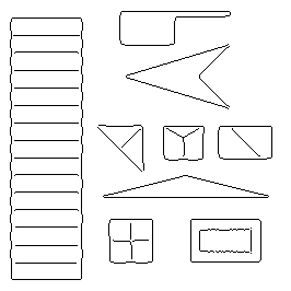

(b)
(c)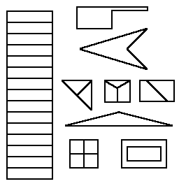

(d)
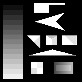
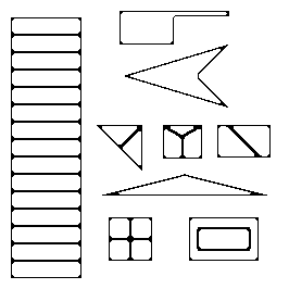
- (a) SUSAN test image used in the paper 'SUSAN - A new approach to low level image processing' by Smith S.M. and Brady J.M. in International J. Computer Vision 23 (1997) 45-78.
- (b) Canny edge detection applied to the SUSAN Test image.
- (c) SUSAN edge detection applied to the SUSAN Test image with parameter t=10.
- (d) Our edge detector applied to the SUSAN Test image using l=0.1, it =1 and thres =1.

iv) SUSAN test image with an affine perturbation
(a)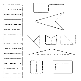

(b)
(c)

(d)
- (a) SUSAN test image with the addition of the affine function ƒ(i,j)=5∙(i-j).
- (b) Canny edges.
- (c) SUSAN edges with parameter t=10.
- (d) Our edges for l=0.1, it =1 and thres =1.

v) SUSAN test image with a quadratic perturbation
(a)

(b)
(c)

(d)
- (a) SUSAN test image with the addition of the quadratic function ƒ(i,j)=(j-255)²-(i-255)².
- (b) Canny edges.
- (c) SUSAN edges with parameter t=10.
- (d) Our edges for l=0.1, it =1 and thres =7.

vi) Test image with Gaussian noise
(a)

(b)
(c)

(d)
- (a) Test image with the addition of Gaussian noise.
- (b) Canny edges with s=3.
- (c) The edges displayed in this picture have been obtained by applying twice the SUSAN algorithm. When applied the first time, the SUSAN algorithm filters the Gaussian noise and returns a binary image with sligthly perturbed edges. By applying again the SUSAN algorithm on the filtered image, one is then able to extract the edges of the background picture.
- (d) Our edges for l=0.001, it =1 and thres =90.

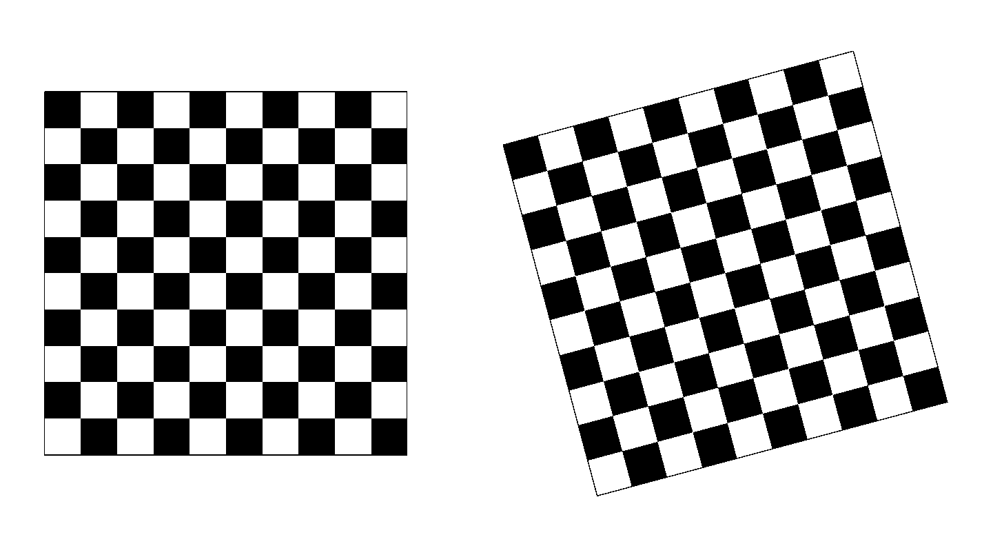
vii) Chessboard test image
(a)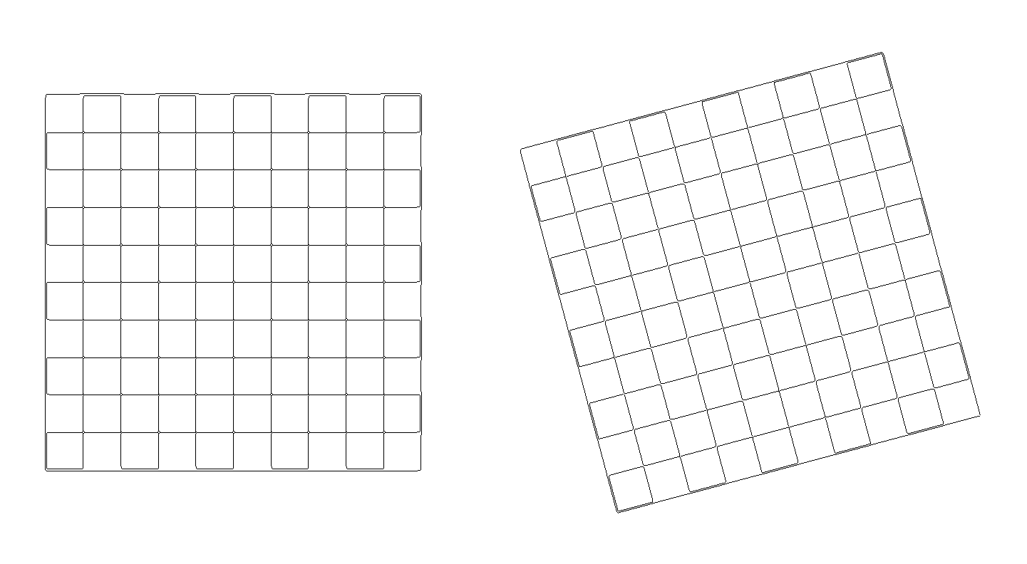

(b)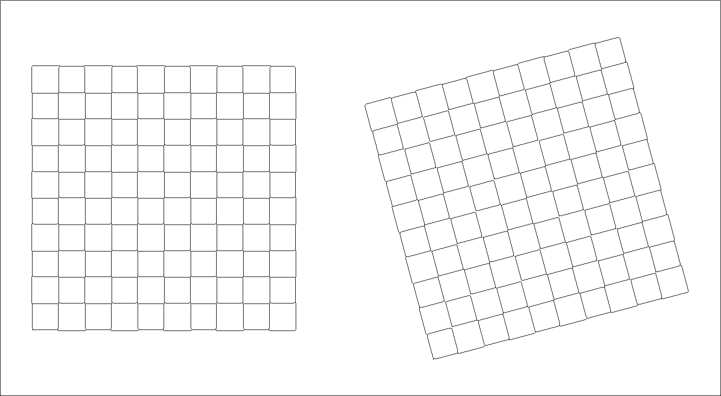

(c)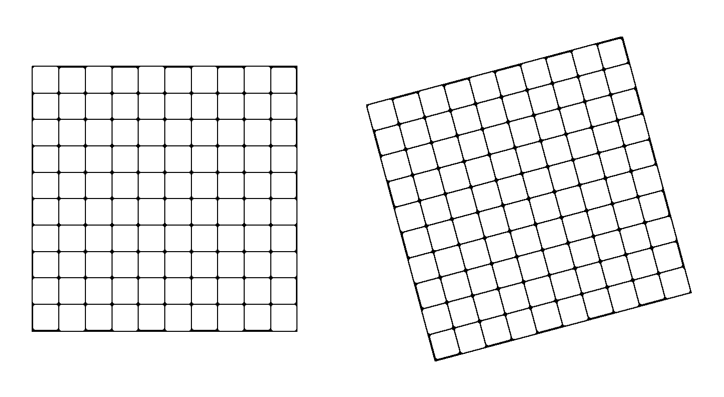

(d)
- (a) Chessboard test image.
- (b) Canny edges.
- (c) SUSAN edge detector.
- (d) Our edges for l=0.1, it =10 and thres =190.