
-
Image Smoothing
-
-
By image smoothing we mean, in general, a transformation that filters the spatial high frequency content of the image. Such transformations are a necessary part of image processing in at least two situations: An image needs to be smoothed before features can be extracted, and images must be smoothed before they are sampled. Common low pass filters are the Butterworth and the Gaussian which consist in modifying the Fourier transform of the image and then computing the inverse transform to obtain the processed result. The main
drawback of using Fourier transform based filters is the poor spatial
localization they provide. Alternative approaches have been proposed based, for instance, on the wavelet transforms
and on minimizing a smooth norm of the error augmented of a regularizing term measuring the total varaition of the restored image.
For more details on the frequency domain filtering refer to the book Digital Image Processing by R. C. Gonzalez and R. E. Woods, Pearson International Edition, 3rd Ed, 2008, whereas for a general review of image denoising algorithms refer to 'A review of image denoising algorithms, with a new one' by A. Buades, B. Coll and J.M. Morel in SIAM Multiscale Model. Simul. 4 (2005) 490-530.
This page displays applications of our smoothing transformation which operates directly on the image in its spatial domain and comparison with the TV based denoising algorithm proposed in 'Nonlinear total variation based noise removal algorithms' by L. Rudin, S. Osher and E. Fatemi in Physica D 60 (1992) 259-268.
-
By image smoothing we mean, in general, a transformation that filters the spatial high frequency content of the image. Such transformations are a necessary part of image processing in at least two situations: An image needs to be smoothed before features can be extracted, and images must be smoothed before they are sampled. Common low pass filters are the Butterworth and the Gaussian which consist in modifying the Fourier transform of the image and then computing the inverse transform to obtain the processed result. The main
drawback of using Fourier transform based filters is the poor spatial
localization they provide. Alternative approaches have been proposed based, for instance, on the wavelet transforms
and on minimizing a smooth norm of the error augmented of a regularizing term measuring the total varaition of the restored image.
For more details on the frequency domain filtering refer to the book Digital Image Processing by R. C. Gonzalez and R. E. Woods, Pearson International Edition, 3rd Ed, 2008, whereas for a general review of image denoising algorithms refer to 'A review of image denoising algorithms, with a new one' by A. Buades, B. Coll and J.M. Morel in SIAM Multiscale Model. Simul. 4 (2005) 490-530.
- i) Results on the proposed smoothing transformation
-
(a)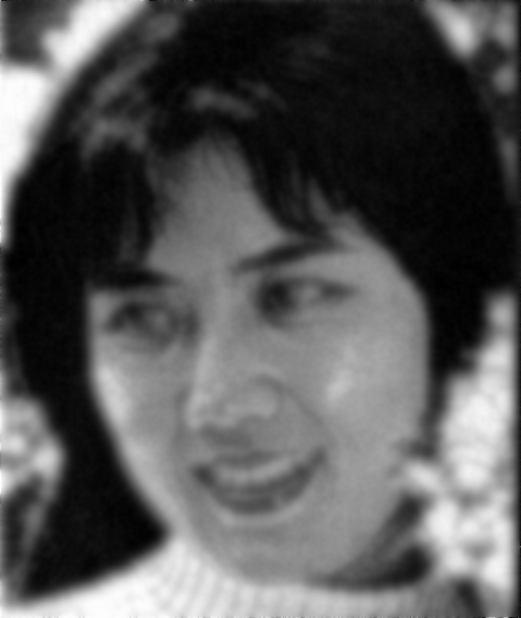
(b) -
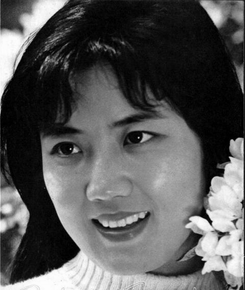
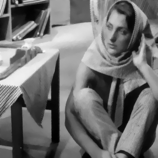
- (a) Original image with size 479×568.
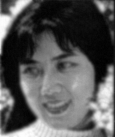
- (b) Smoothed image
-

(a)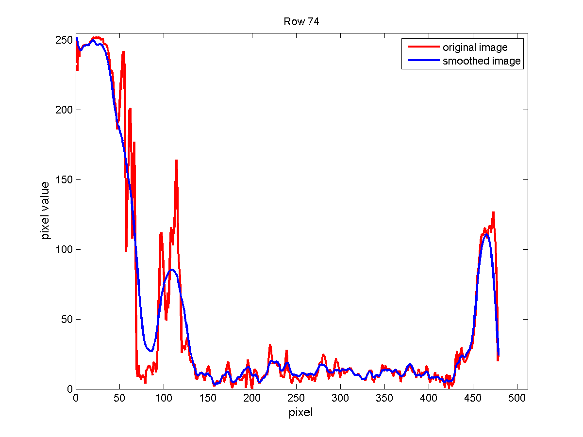
(b) -
- (a) Smoothed image with marked scan line.
-
(b) Pixel values diagram across the scan line.

-
-

(a)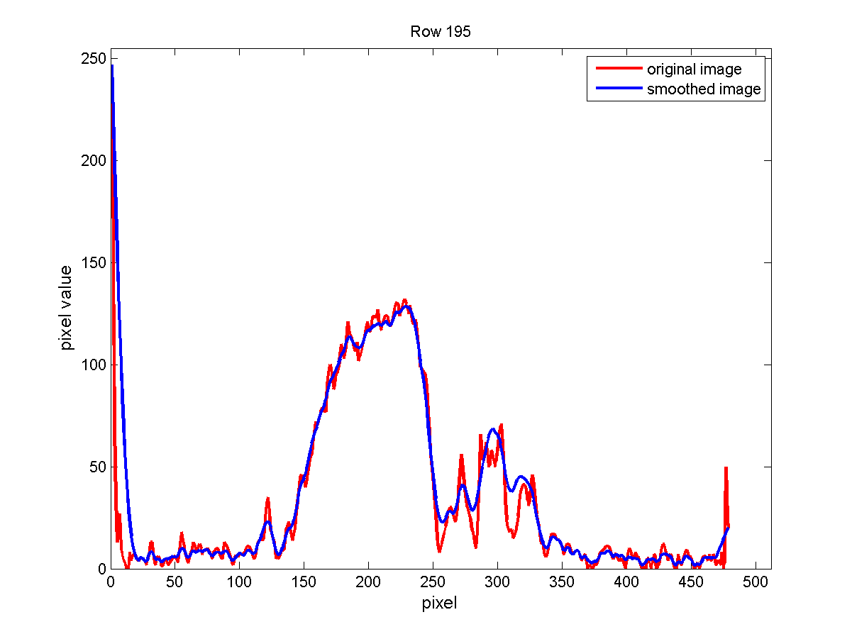
(b) -
- (a) Smoothed image with marked scan line.
-
(b) Pixel values diagram across the scan line.
-
-

(a)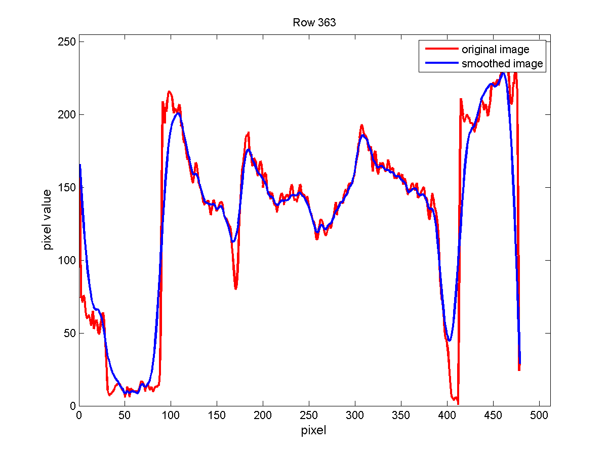
(b) -
- (a) Smoothed image with marked scan line.
-
(b) Pixel values diagram across the scan line.
-
-

(a)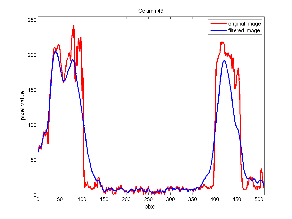
(b) -
- (a) Smoothed image with marked scan line.
-
(b) Pixel values diagram across the scan line.
-
-

(a)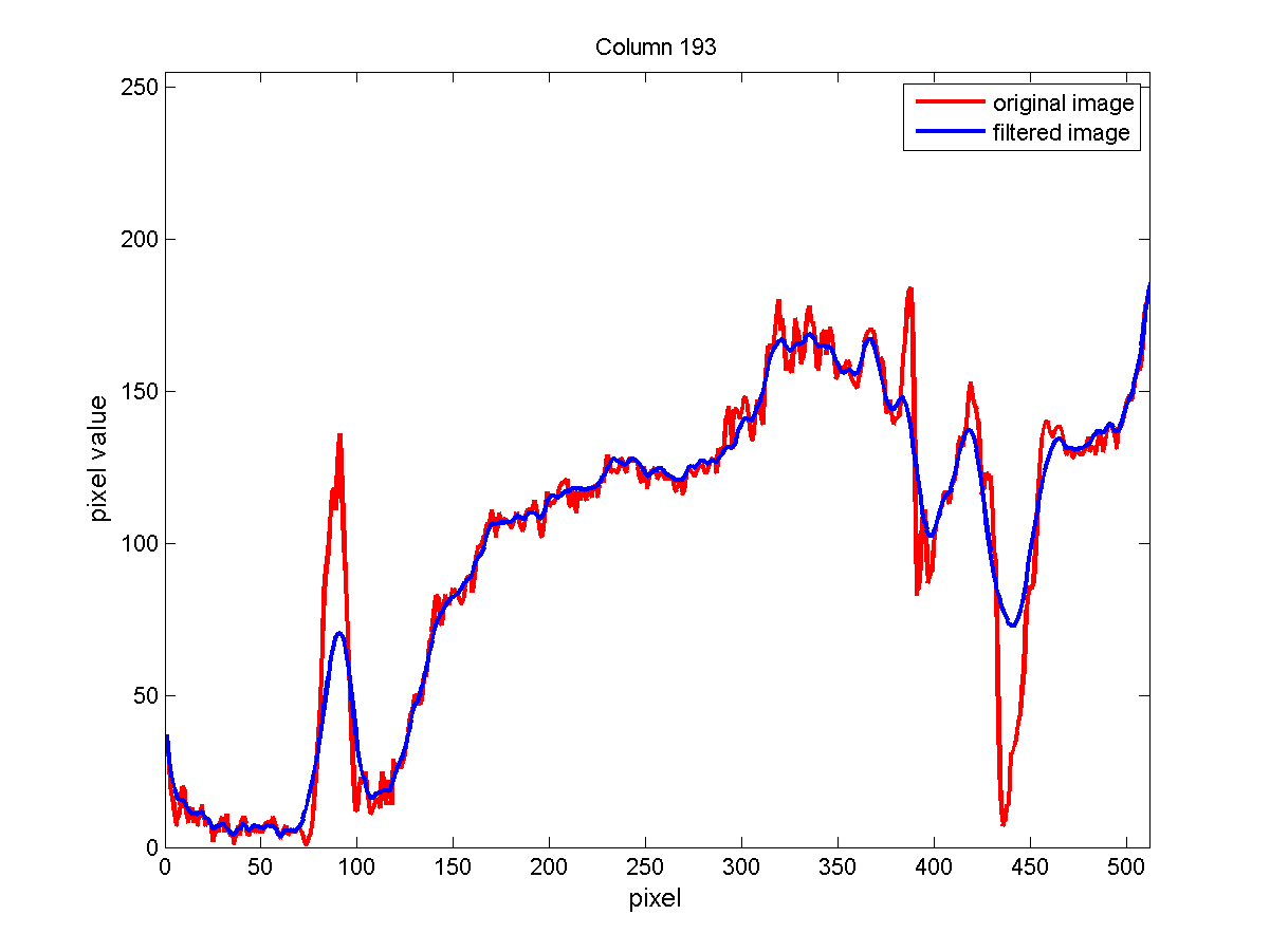
(b) -
- (a) Smoothed image with marked scan line.
-
(b) Pixel values diagram across the scan line.
-
-
(a)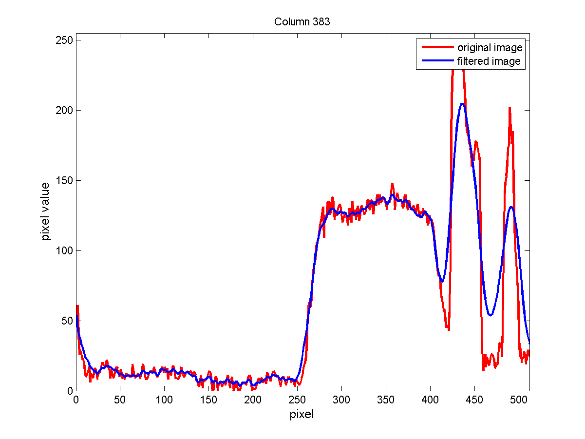
(b) -
- (a) Smoothed image with marked scan line.
-
(b) Pixel values diagram across the scan line.
- ii) Comparison with a TV based smoothing transformation
-

(a)
(b) -
(c)
(d) -
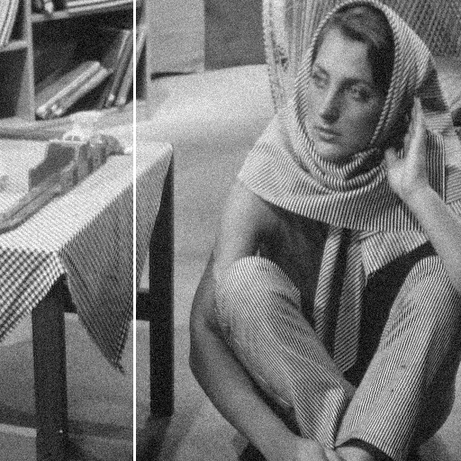
- (a) 8-bit gray scale input image F with size 512×512.
- (b) Image with added Gaussian noise with standard variance s equal to 255×0.05=12.5. That is, let F be the noise free image, in these experiments the noisy image ƒ has been obtained as ƒ=F+srandn(size(F)).
- (c) Restored image obtained by minimizing the functional ∫Ω|∇u|dx+λ/2 ∫Ω(u-ƒ)2dx with ƒ the input noisy image and l set equal to 12. For the minimization, the Chambolle's algorithm described in 'An algorithm for total variation minimization and applications' by A. Chambolle in J. Math. Imag. Vision 20 (2004) 89-97, has been used.
- (d) Smoothed image obtained with our transformation
-
(a)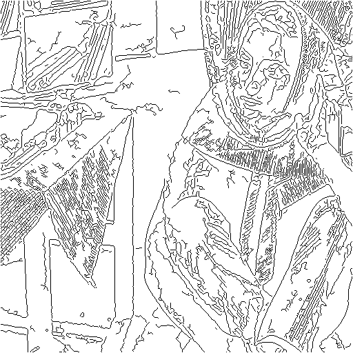
(b) -
(c)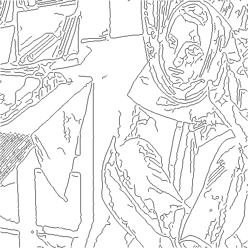
(d) -
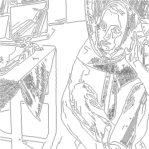
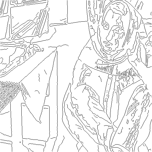
- (a) Canny edges for the original image.
- (b) Canny edges for the noisy image.
- (c) Canny edges for the TV restored image.
-
(d) Canny edges for the restored image by the proposed transformation.
-

(a)
(b)
(c) -
-
(d) -
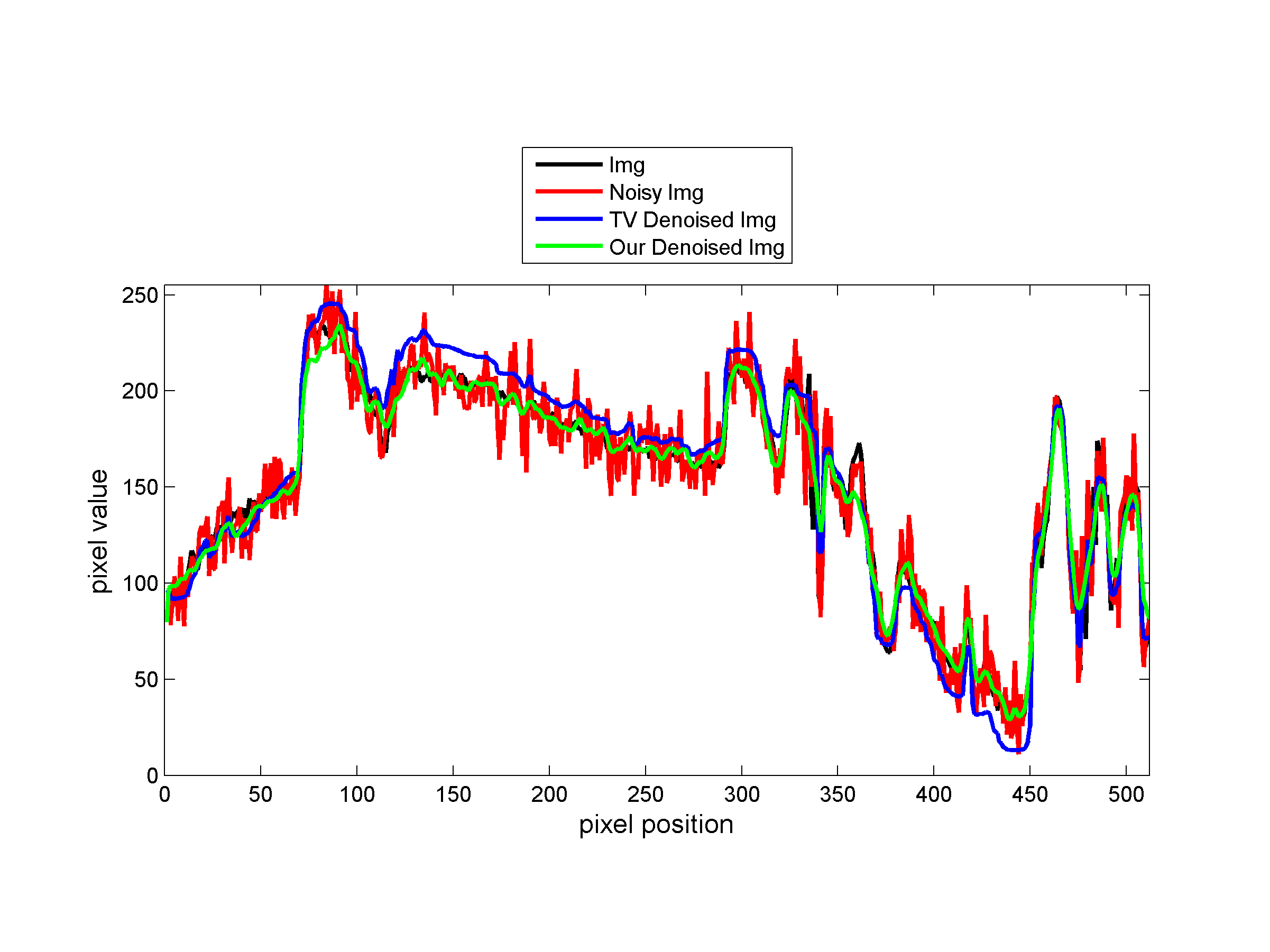
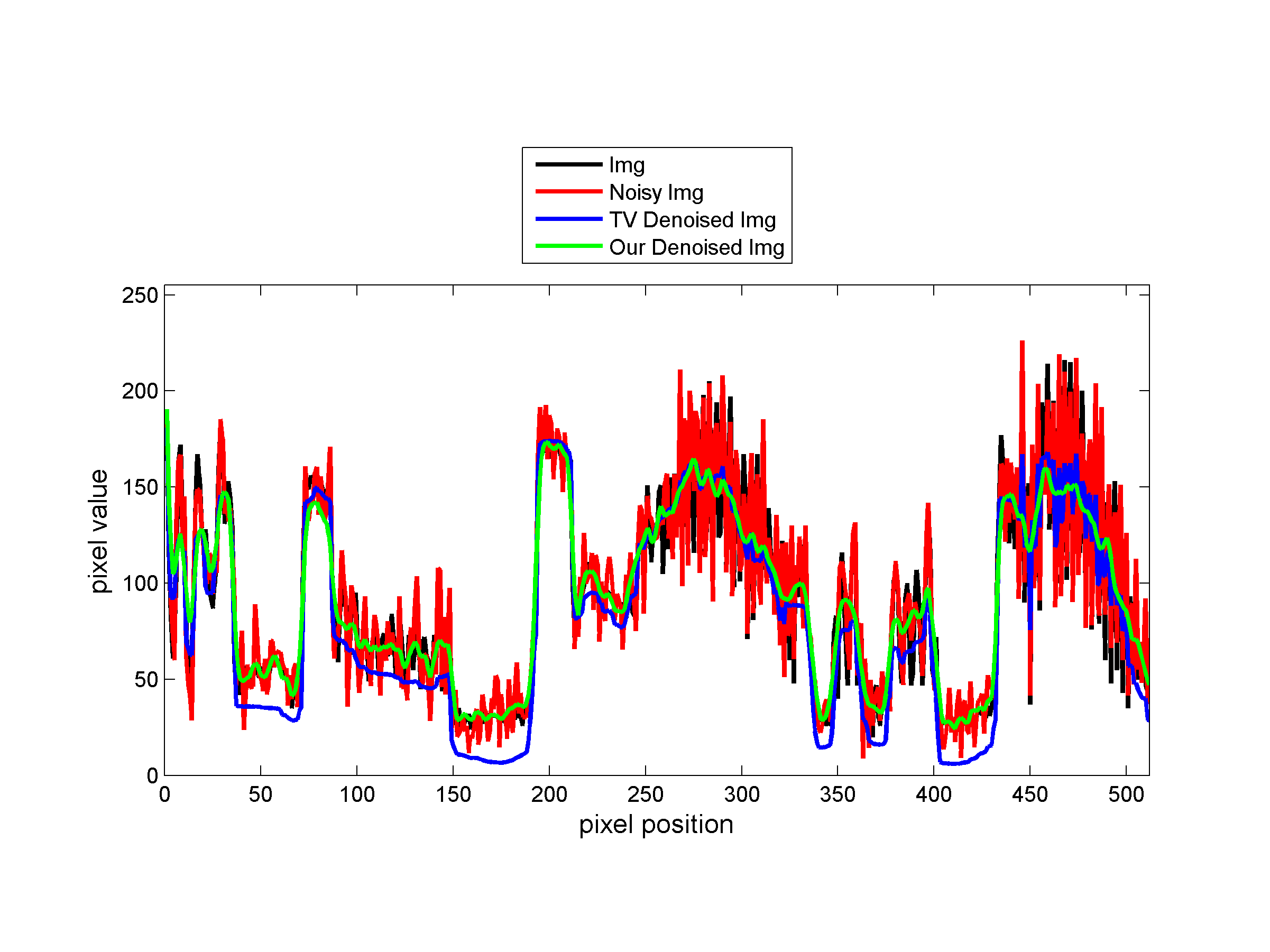
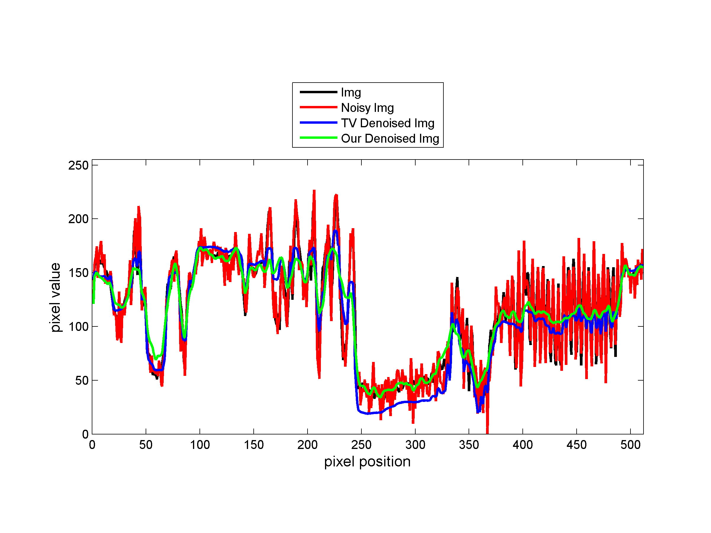
- (a) Noisy image with indication of the scan line.
- (b) TV restored image with indication of the scan line.
- (c) Smoothed restored image with indication of the scan line.
-
(d) Pixel values diagram across the scan line.
-

(a)
(b)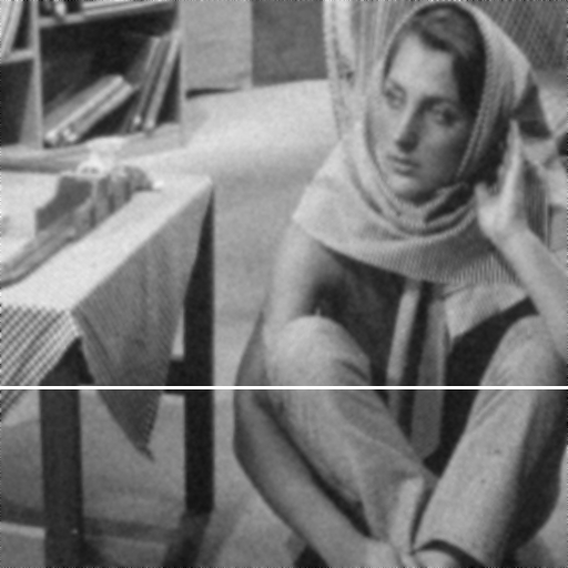
(c) -
-
(d) -
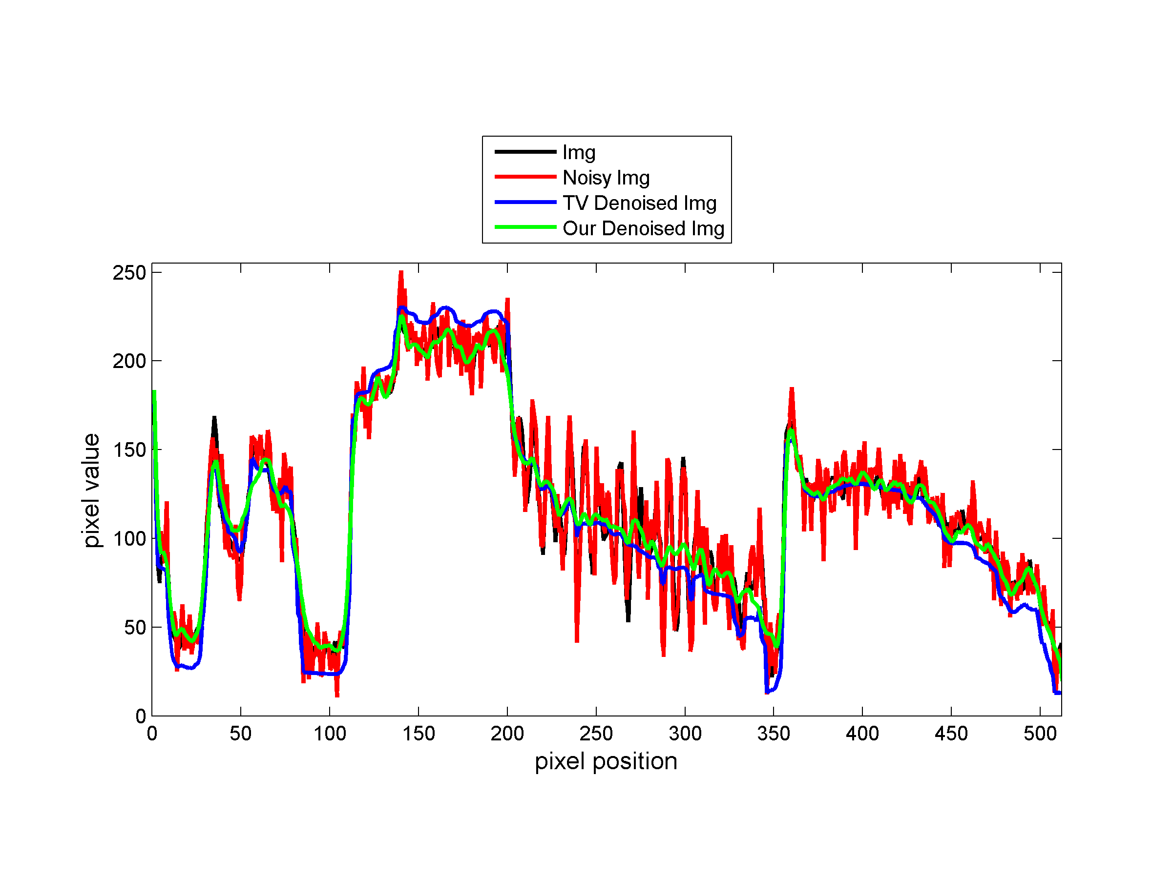
- (a) Noisy image with indication of the scan line.
- (b) TV restored image with indication of the scan line.
- (c) Smoothed restored image with indication of the scan line.
-
(d) Pixel values diagram across the scan line.
-
(a)
(b)
(c) -
-
(d) -
- (a) Noisy image with indication of the scan line.
- (b) TV restored image with indication of the scan line.
- (c) Smoothed restored image with indication of the scan line.
-
(d) Pixel values diagram across the scan line.
-

(a)
(b)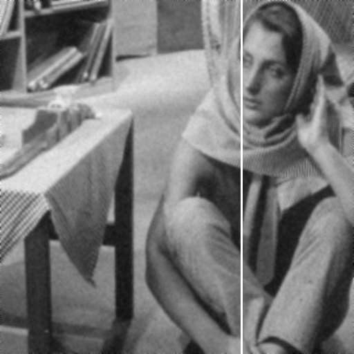
(c) -
-
(d) -
- (a) Noisy image with indication of the scan line.
- (b) TV restored image with indication of the scan line.
- (c) Smoothed restored image with indication of the scan line.
-
(d) Pixel values diagram across the scan line.
Home | Profile | Applications |
Terms of Service | Contact Us
© 2011 KEA All Rights Reserved